QGIS Setup and Export Walkthrough

Quick reference

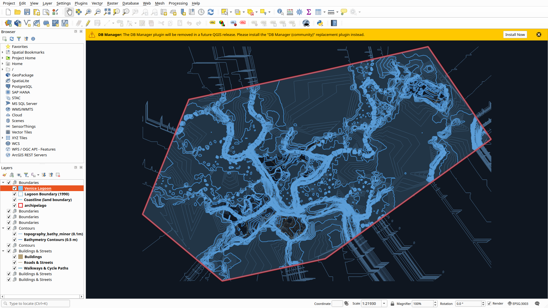
• Recommended version: QGIS 4.2.x "Belém do Pará" (latest release). This matches the studio project files and the version used to prepare the course data.
• Stable alternative: QGIS 3.44.x "Solothurn" (Long Term Release). Choose this if you want maximum reliability over new features.
• Download: https://www.qgis.org/download/
• Installation guide: https://www.qgis.org/resources/installation-guide
• Studio coordinate systems: the course data mixes three CRS. Regione Veneto vector layers are Monte Mario Gauss-Boaga, mostly EPSG:3003 (zone 1) with some EPSG:3004 (zone 2); DEM and bathymetry rasters are EPSG:32633 (WGS 84 / UTM zone 33N); OpenStreetMap data is EPSG:4326. QGIS reprojects every layer to the project CRS on the fly, so pick the CRS of your main layers and the rest line up automatically.

1. Install QGIS

QGIS is free, open source, and runs on Windows, macOS, and Linux.

macOS

1. Go to the download page and, under "Download for macOS", choose "Latest Release (4.2)".
2. Open the downloaded `.dmg` file.
3. Drag the QGIS icon into the Applications folder.
4. On first launch, right-click the app and choose Open. macOS may warn about an unidentified developer; choose Open again to proceed.

Windows

1. On the download page, under "Download for Windows", choose the "Latest Release installer (4.2)" or the OSGeo4W network installer.
2. Run the installer and accept the defaults.
3. Launch QGIS Desktop from the Start menu.

Linux

Follow the repository instructions on the download page for your distribution. Do not install from a flatpak or snap if you need to run QGIS plugins.

2. Start a new project

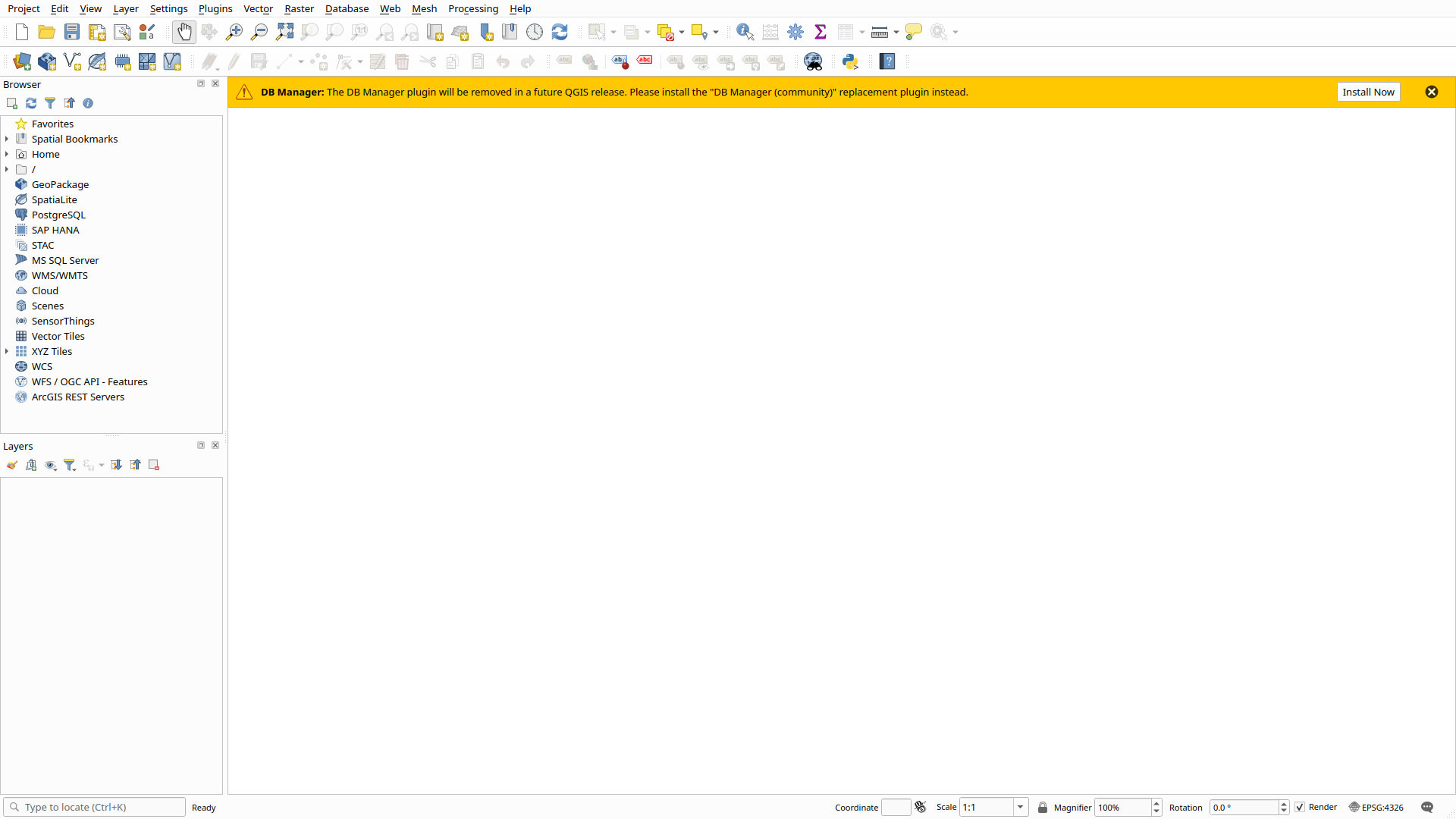
1. Open QGIS.
2. Project → New.
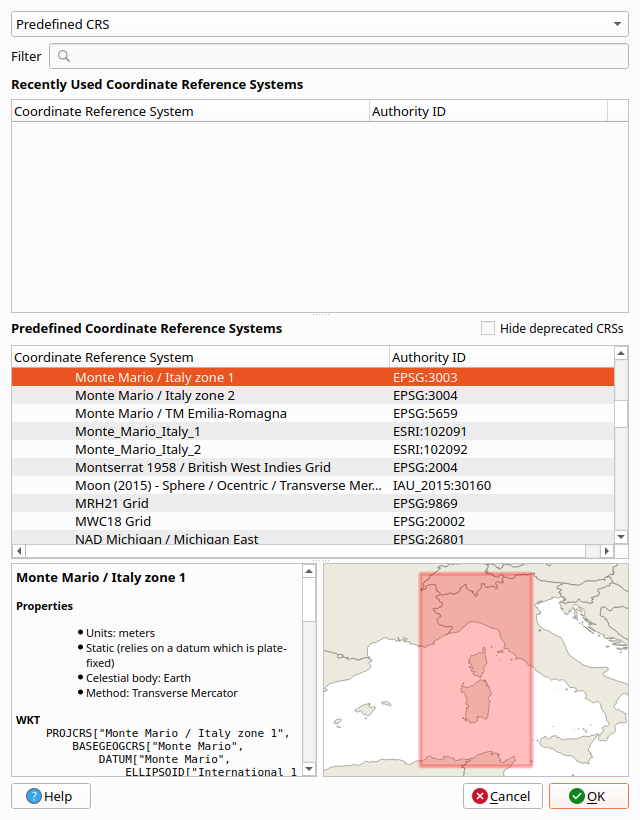
3. Set the coordinate reference system (CRS): Project → Properties → CRS. For the Regione Veneto vector workflows in this tutorial, set EPSG:3003 Monte Mario / Italy zone 1. If you are working with latitude and longitude data, set EPSG:4326 (WGS 84). If your main layers are the DEM or bathymetry rasters, set EPSG:32633 (WGS 84 / UTM zone 33N) instead — see the note below.
4. Save the project with Project → Save. QGIS saves projects as `.qgz` files, which bundle the map and its styling in a single compressed file.

The CRS is how QGIS places data on the map. Every layer must have a known CRS, and QGIS reprojects layers to the project CRS automatically, so data from different sources lines up correctly.

Venice sits at roughly 12.34°E, just east of the 12°E boundary, so its true UTM zone is 33N — EPSG:32633 (WGS 84) or EPSG:25833 (ETRS89) — not 32N. The "UTM zone 32N" sometimes quoted for Venice comes from global elevation tiles (TINITALY, Copernicus) that use 32N as a whole-Italy coverage convention, not from Venice's actual zone. The Regione Veneto vectors are Monte Mario Gauss-Boaga, mostly zone 1 (EPSG:3003) with a smaller set in zone 2 (EPSG:3004); the DEM and bathymetry rasters are EPSG:32633. Two bathymetry files, `bathy_5m.tif` and `venice_merged_5m.tif`, carry no embedded CRS — when you load them, assign EPSG:32633 (right-click the layer → Layer CRS → Set Layer CRS) or QGIS will place them incorrectly.

3. Import data layers

QGIS works with two families of data: vector and raster.

Vector layers

Vector data is geometry with attributes. Three types:

• Point: a single location (a well, a tree, a sensor).
• Line: connected points (roads, rivers, contours, paths).
• Polygon: enclosed areas (buildings, parcels, the lagoon itself).

Common vector formats: Shapefile (`.shp`), GeoPackage (`.gpkg`), GeoJSON (`.geojson`), KML, and DXF.

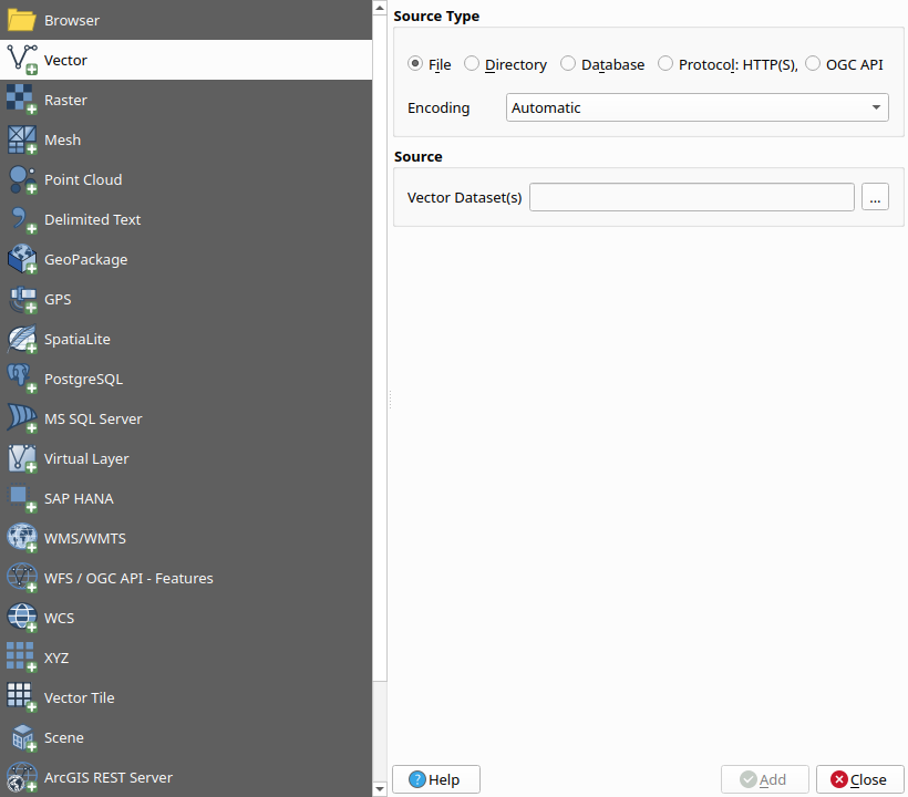
To add a vector layer: Layer → Add Layer → Add Vector Layer, then browse to the file. You can also drag and drop a file from your file browser into the map canvas.

Raster layers

Raster data is a grid of cells, each holding one value. Three types:

• Continuous raster: each cell is a measurement (elevation DEM, bathymetry, slope). You style these with a color ramp.
• Thematic raster: each cell is a class (land cover, zoning). You style these with one color per class.
• Imagery raster: photographs (orthophoto, satellite imagery). You display these as red, green, and blue bands.

Common raster formats: GeoTIFF (`.tif`), JPEG2000, ASCII grid, ECW.

To add a raster layer: Layer → Add Layer → Add Raster Layer, then browse to the file.

Add the 2024 AGEA orthophoto from the web (WMS)

The Regione Veneto serves its 2024 aerial orthophoto mosaic, the AGEA 2024 orthofoto at 20 cm ground resolution, as a free web map service. This is the sharpest aerial imagery available for the lagoon, and it streams straight into QGIS, so there is no 20+ GB download. You do need an internet connection.

1. Layer → Add Layer → Add WMS/WMTS Layer…. (Or open the Data Source Manager with Layer → Data Source Manager and choose WMS/WMTS on the left.)
2. Click New to create a connection. Give it a name such as `Regione Veneto WMS` and paste this URL:

`https://idt2-geoserver.regione.veneto.it/geoserver/ows`

1. Click OK, then click Connect. QGIS downloads the service's layer list; this can take a few seconds.
2. Expand the service entry and find the 2024 orthophoto, listed as AGEA 2024 ortofoto (service layer `rv:ortofoto_agea_2024`). Select only that layer, not the whole service.
3. Click Add, then Close. The orthophoto appears in the Layers panel and on the canvas.
4. Drag it near the bottom of the layer list so your vector overlays (contours, buildings, section lines) draw on top of it.

Notes:

• The service delivers the mosaic in EPSG:3003. QGIS reprojects it on the fly to your project CRS, so it lines up with both the EPSG:3003 vector workflows and the EPSG:32633 raster workflows.
• As you zoom, QGIS requests the tiles it needs and caches them locally, so revisiting an area is faster the second time.
• The WMS stops at the tiles already cached once you lose your connection. The studio project file (`venice_lagoon_studio_styled.qgz`) already includes this layer under the name AGEA 2024 ortofoto (20cm, live); this section covers building it yourself in a fresh project. If you need an offline background, a 50 cm 2018 clip of the northern lagoon is available from the studio data.

4. Style layers

Style a vector layer

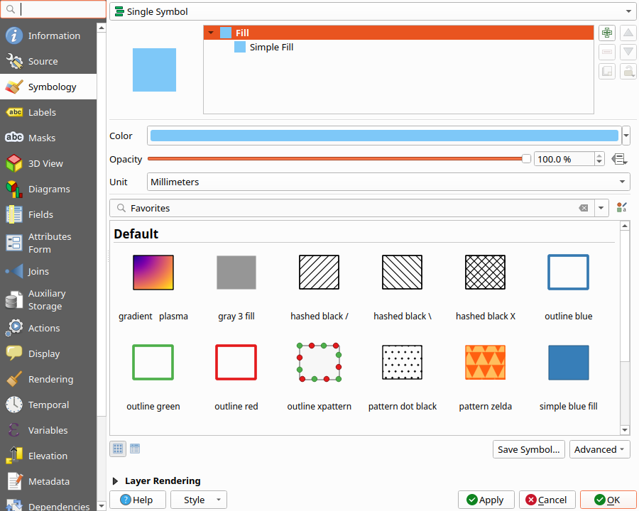
1. Right-click the layer and choose Properties → Symbology.
2. Pick a renderer from the top dropdown:

• Single Symbol: one style for every feature.
• Categorized: one color per value of a field (for example, one color per land use type).
• Graduated: a color ramp across numeric values (for example, building height or flood depth).

1. Set the symbol. For a polygon, set the fill color and the stroke. For a line, set the color and width. For a point, set the size and color.

Style a raster layer

1. Right-click the layer and choose Properties → Symbology.
2. For a continuous raster (a DEM or bathymetry), set Render type to Singleband pseudocolor, choose a color ramp, and set the min and max values.
3. For imagery, set Render type to Multiband color and assign the red, green, and blue bands.

5. Mask or crop a layer to a polygon

To limit a layer to a study area, clip it with a polygon.

Make a polygon to clip with (no data source needed)

If you do not have a clip polygon yet, draw one directly in QGIS:

1. Layer → Create Layer → New Temporary Scratch Layer.
2. Set the geometry type to Polygon and the CRS to EPSG:3003 (or match your project CRS), then click OK.
3. Click the Toggle Editing pencil icon, then click Add Polygon Feature.
4. Click points on the map to trace your study area, then right-click to finish the shape.
5. Enter a name for the feature and click OK. Click the pencil icon again to save and stop editing.

The new layer appears in the Layers panel. Use it as the mask layer or overlay layer in the tools below.

Crop a raster to a polygon (mask)

1. Raster → Extraction → Clip Raster by Mask Layer.
2. Set Input layer to your raster and Mask layer to your polygon.
3. Assign a nodata value (for example -9999) so cells outside the polygon are empty, then Run.

Clip a vector to a polygon

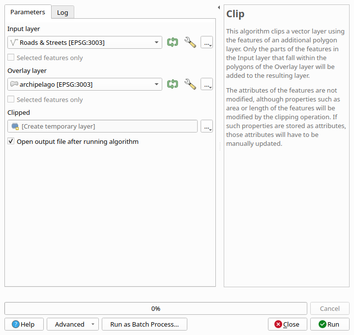
1. Vector → Geoprocessing Tools → Clip.
2. Set Input layer to your vector and Overlay layer to your polygon, then Run. The output keeps only the features that fall inside the polygon.

Both tools are also in the Processing Toolbox (open it with Processing → Toolbox) under the same names.

6. Set up a sheet layout for printing

The Print Layout is where you compose a finished map sheet.

1. Project → New Print Layout, then give the layout a name.
2. In the layout window, add the pieces you need from the toolbar on the left:

• Add Map: draw a rectangle; this is the map frame.
• Add Scale Bar.
• Add Legend.
• Add North Arrow.
• Add Label: for the title, source, and author.

1. Select the map item and, in Item Properties on the right, set the scale, or use Set map extent to match main canvas extent to match what is on screen.
2. Set the page size: right-click the page and choose Page Properties, then set the size to A3 or A4 (landscape or portrait).
3. Export the sheet: Layout → Export as Image (PNG) or Layout → Export as PDF.

7. Export to DXF or AI

Export to DXF (for AutoCAD and Rhino)

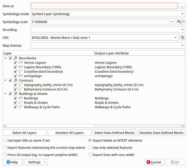
1. Project → Import/Export → Export Project to DXF.
2. Choose the layers to export and a destination CRS. Use EPSG:3003 (or your project CRS).
3. Save. The `.dxf` keeps each QGIS layer as a separate DXF layer. If your source data carries Z values (elevation), those Z values survive in the DXF as 3D geometry.

Export to Adobe Illustrator

QGIS does not write `.ai` files directly. Use one of two routes:

• Route A: SVG (recommended): in the Print Layout, choose Layout → Export as SVG, then open the `.svg` in Illustrator. Labels, legend, and linework stay fully editable vector objects.
• Route B: PDF: in the Print Layout, choose Layout → Export as PDF, then open the `.pdf` in Illustrator. This preserves type and styling but can import less cleanly than SVG.

Tip: for a clean Illustrator file, export from a Print Layout at a fixed scale. Do not export the raw project view; it loses the sheet framing, scale bar, and legend.

Venice data notes

• The Regione Veneto lagoon data uses Monte Mario projections. Zone 1 is EPSG:3003 and zone 2 is EPSG:3004. Set the project CRS to EPSG:3003 and let QGIS reproject zone 2 layers on the fly. In the course archive the zone 1 files are the majority (88 of 131 shapefiles); zone 2 appears in files such as `cb13_acqua` and `batimetria_mare_2011`.
• DEM and bathymetry rasters (`Lagune2013_*.tif`, `bathy_5m.tif`, `venice_merged_5m.tif`, the TINITALY DEMs) are WGS 84 / UTM zone 33N, EPSG:32633 — not 32N.
• `bathy_5m.tif` and `venice_merged_5m.tif` have no CRS tag embedded. If a raster lands in the wrong place or QGIS reports an unknown CRS, assign EPSG:32633 manually.
• The "0.5 m" bathymetry and topography datasets are vector contour lines, not a raster. If you need a continuous surface, interpolate a DEM from the contours (ask in studio).
• OpenStreetMap data (from Geofabrik) is in WGS 84 (EPSG:4326). Reproject it to EPSG:3003 when you combine it with the lagoon data.
• The sharpest aerial imagery for the lagoon is the AGEA 2024 orthophoto (20 cm), streamed as a live WMS from the Regione Veneto IDT2 server. Section 3, "Add the 2024 AGEA orthophoto from the web (WMS)", walks through adding it. For offline work, the 2018 50 cm northern lagoon clip is available from the studio data.